Syntax
>>> STEADY-STATE (SAVE) (: (-)time_step)
Parent Command
>> OPTION
Subcommand
-
Description
This command allows TOUGH2 to reach steady state prior to or after a transient simulation. This option can be used to calibrate against steady-state data (only or in combination with transient data), or to reach an equilibrium as initial conditions for a subsequent transient simulation. Note that a transient TOUGH2 simulation must be performed to reach steady state which is usually indicated by one of the following convergence failures:
– too many time steps converged on a single Newton-Raphson iteration (see command >>> CONSECUTIVE);
– convergence failure followed by two time steps converging on a single Newton- Raphson iteration;
– too many time step reductions (see command >>> REDUCTION);
– maximum number of time steps reached (TOUGH2 variable MCYC);
– maximum simulation time reached (TOUGH2 variable TIMAX);
– maximum time step size reached (use a colon on the command line followed by max_time_step to select a maximum time step size. The time_step must be smaller than TOUGH2 variable DELTMX)
-minimum time step size reached (use a colon on the command line followed by a negative time_step to select a minimum time step size, suggesting convergence problems that are assumed to indicate steady-state conditions are reached).
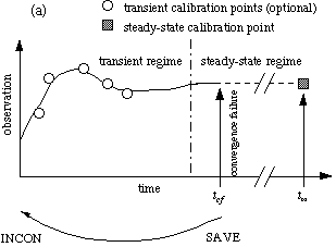
iTOUGH2 usually stops if a TOUGH2 run terminates due to one of the above mentioned convergence failures (see command >>> INCOMPLETE). If command >>> STEADY-STATE is present, however, it accepts convergence failures and proceeds with the inversion. Inversions involving steady-state runs can be greatly accelerated by using keyword SAVE on the command line. After the first steady-state run has been completed, iTOUGH2 takes the steady-state conditions stored on file SAVE as the initial condition (file INCON) for the next TOUGH2 run, sets the initial time step to the (usually large) last time step of the previous simulation, and updates the parameters. Since the parameter set is changed only slightly between subsequent TOUGH2 runs, the new steady state is usually reached within a few additional time steps. This option should not be used if also calibrating against transient data preceding the steady-state data point. Assuming that calibration against steady-state data is to be performed, a steady-state calibration time tINF should be specified at a very late point in time (i.e., beyond the transient phase of the simulation), and the same time should be assigned to the observed steady-state data point in block >>>> DATA. (In addition to the steady-state point, one might also specify calibration points during the transient phase). The TOUGH2 simulation proceeds until a convergence failure occurs at an unknown point in time tCF. The primary variables at that point are written to file SAVE and reused as initial conditions for the subsequent TOUGH2 run (only if keyword SAVE is present). Then, the calculated system state at time tCF is compared to the steady-state data point at time tINF (make sure that tINF is always greater than tCF, e.g., set tINF=1.0E20).
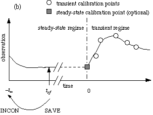
 The second application of the steady-state option is the following. If a steady-state regime is to precede a transient regime within a single simulation (e.g., to assure initial conditions are at equilibrium, a state that depends on the parameters to be estimated), a negative starting time -tINF (TOUGH2 variable TSTART) must be specified. Ensure that |-tINF| is larger than the duration required to reach steady state, e.g., -tINF = -1.0E20. The TOUGH2 simulation proceeds until a convergence failure occurs at an unknown point in time tCF creating the steady-state regime. The primary variables at that point are written to file SAVE to be used as initial conditions for the subsequent TOUGH2 run (only if keyword SAVE is present). The simulation time is then set to zero, and the transient regime of the simulation is initiated. This requires that boundary conditions are changed at time zero, e.g., by starting injection or withdrawal, or by changing Dirichlet-type boundary conditions (see command >> RESTART TIME). (Note that if transient data are combined with steady-state data, the standard deviation of the steady-state data point may have to be decreased substantially to outweigh the large number of transient points.)
 Example
> OBSERVATION
>> steady-state point in TIME: 1 (= t_inf)
1.0E20
>> PRESSURE
>>> ELEMENT: FDF76
>>>> DATA
1.0E20 1.354E5
>>>> DEVIATION: 0.05E5
<<<<
<<<
<<
> COMPUTATION
>> OPTION
>>> allow STEADY-STATE, use SAVE file for restart
<<<
>> CONVERGEnce criteria
>>> Presume steady-state if : 5 CONSECUTIVE time steps converge on ITER=1
>>> number of ITERATIONS: 5
<<<
<<
<
See Also
>> RESTART TIME | >>> CONSECUTIVE | >>> INCOMPLETE | >>> REDUCTION